A slightly longer Lean 4 proof tour

In my previous post, I walked through the task of formally deducing one lemma from another in Lean 4. The deduction was deliberately chosen to be short and only showcased a small number of Lean tactics. Here I would like to walk through the process I used for a slightly longer proof I worked out recently, after seeing the following challenge from Damek Davis: to formalize (in a civilized fashion) the proof of the following lemma:

Lemma. Let ${a_k}$ and ${D_k}$ be sequences of real numbers indexed by natural numbers $k=0,1,dots$ , with $a_k$ non-increasing and $D_k$ non-negative. Suppose also that $a_k leq D_k - D_{k+1}$ for all $k geq 0$ . Then $a_k leq frac{D_0}{k+1}$ for all $k$ .

Here I tried to draw upon the lessons I had learned from the PFR formalization project, and to first set up a human readable proof of the lemma before starting the Lean formalization – a lower-case “blueprint” rather than the fancier Blueprint used in the PFR project. The main idea of the proof here is to use the telescoping series identity

$displaystyle sum_{i=0}^k D_i - D_{i+1}=D_0 - D_{k+1}.$

Since $D_{k+1}$ is non-negative, and $a_i leq D_i - D_{i+1}$ by hypothesis, we have

$displaystyle sum_{i=0}^k a_i leq D_0$

but by the monotone hypothesis on $a_i$ the left-hand side is at least $(k+1) a_k$ , giving the claim.

This is already a human-readable proof, but in order to formalize it more easily in Lean, I decided to rewrite it as a chain of inequalities, starting at $a_k$ and ending at $D_0 / (k+1)$ . With a little bit of pen and paper effort, I obtained

$a_k=(k+1) a_k / (k+1)$

(by field identities)

$=(sum_{i=0}^k a_k) / (k+1)$

(by the formula for summing a constant)

$leq (sum_{i=0}^k a_i) / (k+1)$

(by the monotone hypothesis)

$leq (sum_{i=0}^k D_i - D_{i+1}) / (k+1)$

(by the hypothesis $a_i leq D_i - D_{i+1}$

$=(D_0 - D_{k+1}) / (k+1)$

(by telescoping series)

$leq D_0 / (k+1)$

(by the non-negativity of $D_{k+1}$ ).

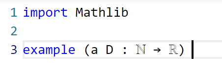
I decided that this was a good enough blueprint for me to work with. The next step is to formalize the statement of the lemma in Lean. For this quick project, it was convenient to use the online Lean playground, rather than my local IDE, so the screenshots will look a little different from those in the previous post. (If you like, you can follow this tour in that playground, by typing in some version of the code displayed below.) I start by importing Lean’s math library, and starting an example of a statement to state and prove:

Now we have to declare the hypotheses and variables. The main variables here are the sequences $a_k$ and $D_k$ , which in Lean are best modeled by functions a, D from the natural numbers ℕ to the reals ℝ. (One can choose to “hardwire” the non-negativity hypothesis into the $D_k$ by making D take values in the nonnegative reals ${bf R}^+$ (denoted NNReal in Lean), but this turns out to be inconvenient, because the laws of algebra and summation that we will need are clunkier on the non-negative reals (which are not even a group) than on the reals (which are a field). So we add in the variables:

Now we add in the hypotheses, which in Lean convention are usually given names starting with h. This is fairly straightforward; the one thing is that the property of being monotone decreasing already has a name in Lean’s Mathlib, namely Antitone, and it is generally a good idea to use the Mathlib provided terminology (because that library contains a lot of useful lemmas about such terms).

One thing to note here is that Lean is quite good at filling in implied ranges of variables. Because a and D have the natural numbers ℕ as their domain, the dummy variable k in these hypotheses is automatically being quantified over ℕ. We could have made this quantification explicit if we so chose, for instance using ∀ k : ℕ, 0 ≤ D k instead of ∀ k, 0 ≤ D k, but it is not necessary to do so. Also note that Lean does not require parentheses when applying functions: we write D k here rather than D(k) (which in fact does not compile in Lean unless one puts a space between the D and the parentheses). This is slightly different from standard mathematical notation, but is not too difficult to get used to.

This looks like the end of the hypotheses, so we could now add a colon to move to the conclusion, and then add that conclusion:

This is a perfectly fine Lean statement. But it turns out that when proving a universally quantified statement such as ∀ k, a k ≤ D 0 / (k + 1), the first step is almost always to open up the quantifier to introduce the variable k (using the Lean command intro k). Because of this, it is slightly more efficient to hide the universal quantifier by placing the variable k in the hypotheses, rather than in the quantifier (in which case we have to now specify that it is a natural number, as Lean can no longer deduce this from context):

At this point Lean is complaining of an unexpected end of input: the example has been stated, but not proved. We will temporarily mollify Lean by adding a sorry as the purported proof:

Now Lean is content, other than giving a warning (as indicated by the yellow squiggle under the example) that the proof contains a sorry.

It is now time to follow the blueprint. The Lean tactic for proving an inequality via chains of other inequalities is known as calc. We use the blueprint to fill in the calc that we want, leaving the justifications of each step as “sorry”s for now:

Here, we “open“ed the Finset namespace in order to easily access Finset‘s range function, with range k basically being the finite set of natural numbers ${0,dots,k-1}$ , and also “open“ed the BigOperators namespace to access the familiar ∑ notation for (finite) summation, in order to make the steps in the Lean code resemble the blueprint as much as possible. One could avoid opening these namespaces, but then expressions such as ∑ i in range (k+1), a i would instead have to be written as something like Finset.sum (Finset.range (k+1)) (fun i ↦ a i), which looks a lot less like like standard mathematical writing. The proof structure here may remind some readers of the “two column proofs” that are somewhat popular in American high school geometry classes.

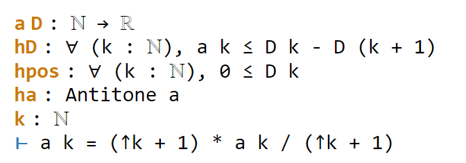
Now we have six sorries to fill. Navigating to the first sorry, Lean tells us the ambient hypotheses, and the goal that we need to prove to fill that sorry:

The ⊢ symbol here is Lean’s marker for the goal. The uparrows ↑ are coercion symbols, indicating that the natural number k has to be converted to a real number in order to interact via arithmetic operations with other real numbers such as a k, but we can ignore these coercions for this tour (for this proof, it turns out Lean will basically manage them automatically without need for any explicit intervention by a human).

The goal here is a self-evident algebraic identity; it involves division, so one has to check that the denominator is non-zero, but this is self-evident. In Lean, a convenient way to establish algebraic identities is to use the tactic field_simp to clear denominators, and then ring to verify any identity that is valid for commutative rings. This works, and clears the first sorry:

field_simp, by the way, is smart enough to deduce on its own that the denominator k+1 here is manifestly non-zero (and in fact positive); no human intervention is required to point this out. Similarly for other “clearing denominator” steps that we will encounter in the other parts of the proof.

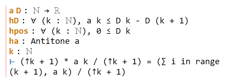
Now we navigate to the next `sorry`. Lean tells us the hypotheses and goals:

We can reduce the goal by canceling out the common denominator ↑k+1. Here we can use the handy Lean tactic congr, which tries to match two sides of an equality goal as much as possible, and leave any remaining discrepancies between the two sides as further goals to be proven. Applying congr, the goal reduces to

Here one might imagine that this is something that one can prove by induction. But this particular sort of identity – summing a constant over a finite set – is already covered by Mathlib. Indeed, searching for Finset, sum, and const soon leads us to the Finset.sum_const lemma here. But there is an even more convenient path to take here, which is to apply the powerful tactic simp, which tries to simplify the goal as much as possible using all the “simp lemmas” Mathlib has to offer (of which Finset.sum_const is an example, but there are thousands of others). As it turns out, simp completely kills off this identity, without any further human intervention:

Now we move on to the next sorry, and look at our goal:

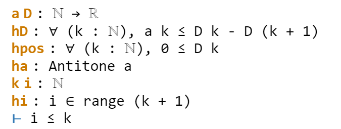
congr doesn’t work here because we have an inequality instead of an equality, but there is a powerful relative gcongr of congr that is perfectly suited for inequalities. It can also open up sums, products, and integrals, reducing global inequalities between such quantities into pointwise inequalities. If we invoke gcongr with i hi (where we tell gcongr to use i for the variable opened up, and hi for the constraint this variable will satisfy), we arrive at a greatly simplified goal (and a new ambient variable and hypothesis):

Now we need to use the monotonicity hypothesis on a, which we have named ha here. Looking at the documentation for Antitone, one finds a lemma that looks applicable here:

One can apply this lemma in this case by writing apply Antitone.imp ha, but because ha is already of type Antitone, we can abbreviate this to apply ha.imp. (Actually, as indicated in the documentation, due to the way Antitone is defined, we can even just use apply ha here.) This reduces the goal nicely:

The goal is now very close to the hypothesis hi. One could now look up the documentation for Finset.range to see how to unpack hi, but as before simp can do this for us. Invoking simp at hi, we obtain

Now the goal and hypothesis are very close indeed. Here we can just close the goal using the linarith tactic used in the previous tour:

The next sorry can be resolved by similar methods, using the hypothesis hD applied at the variable i:

Now for the penultimate sorry. As in a previous step, we can use congr to remove the denominator, leaving us in this state:

This is a telescoping series identity. One could try to prove it by induction, or one could try to see if this identity is already in Mathlib. Searching for Finset, sum, and sub will locate the right tool (as the fifth hit), but a simpler way to proceed here is to use the exact? tactic we saw in the previous tour:

A brief check of the documentation for sum_range_sub’ confirms that this is what we want. Actually we can just use apply sum_range_sub’ here, as the apply tactic is smart enough to fill in the missing arguments:

One last sorry to go. As before, we use gcongr to cancel denominators, leaving us with

This looks easy, because the hypothesis hpos will tell us that D (k+1) is nonnegative; specifically, the instance hpos (k+1) of that hypothesis will state exactly this. The linarith tactic will then resolve this goal once it is told about this particular instance:

We now have a complete proof – no more yellow squiggly line in the example. There are two warnings though – there are two variables i and hi introduced in the proof that Lean’s “linter” has noticed are not actually used in the proof. So we can rename them with underscores to tell Lean that we are okay with them not being used:

This is a perfectly fine proof, but upon noticing that many of the steps are similar to each other, one can do a bit of “code golf” as in the previous tour to compactify the proof a bit:

With enough familiarity with the Lean language, this proof actually tracks quite closely with (an optimized version of) the human blueprint.

This concludes the tour of a lengthier Lean proving exercise. I am finding the pre-planning step of the proof (using an informal “blueprint” to break the proof down into extremely granular pieces) to make the formalization process significantly easier than in the past (when I often adopted a sequential process of writing one line of code at a time without first sketching out a skeleton of the argument). (The proof here took only about 15 minutes to create initially, although for this blog post I had to recreate it with screenshots and supporting links, which took significantly more time.) I believe that a realistic near-term goal for AI is to be able to fill in automatically a significant fraction of the sorts of atomic “sorry“s of the size one saw in this proof, allowing one to convert a blueprint to a formal Lean proof even more rapidly.

One final remark: in this tour I filled in the “sorry“s in the order in which they appeared, but there is actually no requirement that one does this, and once one has used a blueprint to atomize a proof into self-contained smaller pieces, one can fill them in in any order. Importantly for a group project, these micro-tasks can be parallelized, with different contributors claiming whichever “sorry” they feel they are qualified to solve, and working independently of each other. (And, because Lean can automatically verify if their proof is correct, there is no need to have a pre-existing bond of trust with these contributors in order to accept their contributions.) Furthermore, because the specification of a “sorry” someone can make a meaningful contribution to the proof by working on an extremely localized component of it without needing the mathematical expertise to understand the global argument. This is not particularly important in this simple case, where the entire lemma is not too hard to understand to a trained mathematician, but can become quite relevant for complex formalization projects.

>>> Read full article>>>
Copyright for syndicated content belongs to the linked Source : Hacker News – https://terrytao.wordpress.com/2023/12/05/a-slightly-longer-lean-4-proof-tour/